scikit-learn库是当今最流行的机器学习算法库之一
可用来解决分类与回归问题
本章以鸢尾花数据集为例,简单了解八大传统机器学习分类算法的sk-learn实现
传统机器学习算法的原理和推导,学习《统计学习方法》或《西瓜书》
数据集准备 下载数据集 1 iris = sns.load_dataset("iris" )
数据集的查看 pandas.core.frame.DataFrame
(150, 5)
sepal_length
sepal_width
petal_length
petal_width
species
0
5.1
3.5
1.4
0.2
setosa
1
4.9
3.0
1.4
0.2
setosa
2
4.7
3.2
1.3
0.2
setosa
3
4.6
3.1
1.5
0.2
setosa
4
5.0
3.6
1.4
0.2
setosa
<class 'pandas.core.frame.DataFrame'>
RangeIndex: 150 entries, 0 to 149
Data columns (total 5 columns):
# Column Non-Null Count Dtype
--- ------ -------------- -----
0 sepal_length 150 non-null float64
1 sepal_width 150 non-null float64
2 petal_length 150 non-null float64
3 petal_width 150 non-null float64
4 species 150 non-null object
dtypes: float64(4), object(1)
memory usage: 6.0+ KB
sepal_length
sepal_width
petal_length
petal_width
count
150.000000
150.000000
150.000000
150.000000
mean
5.843333
3.057333
3.758000
1.199333
std
0.828066
0.435866
1.765298
0.762238
min
4.300000
2.000000
1.000000
0.100000
25%
5.100000
2.800000
1.600000
0.300000
50%
5.800000
3.000000
4.350000
1.300000
75%
6.400000
3.300000
5.100000
1.800000
max
7.900000
4.400000
6.900000
2.500000
1 2 iris.species.value_counts()
virginica 50
versicolor 50
setosa 50
Name: species, dtype: int64
1 2 3 sns.pairplot(data=iris,hue="species" )
<seaborn.axisgrid.PairGrid at 0x1aac4ed3850>
标签清洗 为了简化问题,我们可以只取花瓣长度和花瓣宽度这两个变量进行鸢尾花的分类
1 2 iris_simple = iris.drop(["sepal_length" , "sepal_width" ], axis=1 ) iris_simple.head()
petal_length
petal_width
species
0
1.4
0.2
setosa
1
1.4
0.2
setosa
2
1.3
0.2
setosa
3
1.5
0.2
setosa
4
1.4
0.2
setosa
标签编码 1 2 3 4 5 from sklearn.preprocessing import LabelEncoderencoder = LabelEncoder() iris_simple["species" ] = encoder.fit_transform(iris_simple["species" ])
fit_transform:
这是一个常用方法,结合了两步操作:
fit:学习类别数据的映射关系(即将每个类别与一个整数标签对应)。
transform:将原始的类别数据转换为对应的数值标签。
petal_length
petal_width
species
0
1.4
0.2
0
1
1.4
0.2
0
2
1.3
0.2
0
3
1.5
0.2
0
4
1.4
0.2
0
...
...
...
...
145
5.2
2.3
2
146
5.0
1.9
2
147
5.2
2.0
2
148
5.4
2.3
2
149
5.1
1.8
2
150 rows × 3 columns
数据集的标准化(本数据集比较接近,实际处理过程中未标准化) 1 2 from sklearn.preprocessing import StandardScalerimport pandas as pd
1 2 3 4 trans=StandardScaler() _iris_simple = trans.fit_transform(iris_simple[["petal_length" ,"petal_width" ]]) _iris_simple=pd.DataFrame(_iris_simple,columns=["petal_length" ,"petal_width" ]) _iris_simple.head()
petal_length
petal_width
0
-1.340227
-1.315444
1
-1.340227
-1.315444
2
-1.397064
-1.315444
3
-1.283389
-1.315444
4
-1.340227
-1.315444
petal_length
petal_width
count
1.500000e+02
1.500000e+02
mean
-8.652338e-16
-4.662937e-16
std
1.003350e+00
1.003350e+00
min
-1.567576e+00
-1.447076e+00
25%
-1.226552e+00
-1.183812e+00
50%
3.364776e-01
1.325097e-01
75%
7.627583e-01
7.906707e-01
max
1.785832e+00
1.712096e+00
构建训练集和测试集(暂时不考虑验证集) 1 2 3 4 from sklearn.model_selection import train_test_splittrain_set, test_set = train_test_split(iris_simple, test_size=0.2 ) test_set.head()
petal_length
petal_width
species
15
1.5
0.4
0
92
4.0
1.2
1
46
1.6
0.2
0
37
1.4
0.1
0
84
4.5
1.5
1
1 2 iris_x_train = train_set[["petal_length" ,"petal_width" ]] iris_x_train.head()
petal_length
petal_width
38
1.3
0.2
52
4.9
1.5
49
1.4
0.2
55
4.5
1.3
117
6.7
2.2
(iris_x_train)不需要 copy():
这里是直接取列(petal_length, petal_width),而没有进一步修改。
(iris_y_train)需要 copy():
目标是将目标变量 species 提取为一个独立的副本,可能会对它进行编码(如 LabelEncoder),因此使用 .copy() 避免无意中修改原始数据。
1 2 iris_y_train = train_set["species" ].copy() iris_y_train.head()
38 0
52 1
49 0
55 1
117 2
Name: species, dtype: int32
1 2 iris_x_test = test_set[["petal_length" ,"petal_width" ]] iris_x_test.head()
petal_length
petal_width
15
1.5
0.4
92
4.0
1.2
46
1.6
0.2
37
1.4
0.1
84
4.5
1.5
1 2 iris_y_test = test_set["species" ].copy() iris_y_test.head()
15 0
92 1
46 0
37 0
84 1
Name: species, dtype: int32
k近邻算法 基本思想:把k个近邻中最常见的类别预测为待预测点的类别
sklearn实现 1 from sklearn.neighbors import KNeighborsClassifier
1 2 3 clf=KNeighborsClassifier() clf
KNeighborsClassifier()
1 2 clf.fit(iris_x_train,iris_y_train)
KNeighborsClassifier()
1 2 3 4 res = clf.predict(iris_x_test) print (res)print (iris_y_test.values)
[0 1 0 0 1 2 1 1 2 1 2 0 2 2 1 0 0 2 0 0 2 2 2 1 1 1 1 2 1 0]
[0 1 0 0 1 2 1 1 2 1 2 0 2 2 1 0 0 2 0 0 2 2 2 1 1 1 1 2 1 0]
D:\software\anaconda\lib\site-packages\sklearn\neighbors\_classification.py:211: FutureWarning: Unlike other reduction functions (e.g. `skew`, `kurtosis`), the default behavior of `mode` typically preserves the axis it acts along. In SciPy 1.11.0, this behavior will change: the default value of `keepdims` will become False, the `axis` over which the statistic is taken will be eliminated, and the value None will no longer be accepted. Set `keepdims` to True or False to avoid this warning.
mode, _ = stats.mode(_y[neigh_ind, k], axis=1)
1 2 encoder.inverse_transform(res)
array(['setosa', 'versicolor', 'setosa', 'setosa', 'versicolor',
'virginica', 'versicolor', 'versicolor', 'virginica', 'versicolor',
'virginica', 'setosa', 'virginica', 'virginica', 'versicolor',
'setosa', 'setosa', 'virginica', 'setosa', 'setosa', 'virginica',
'virginica', 'virginica', 'versicolor', 'versicolor', 'versicolor',
'versicolor', 'virginica', 'versicolor', 'setosa'], dtype=object)
1 2 3 accuracy = clf.score(iris_x_test,iris_y_test) print ("预测正确率:{:.0%}" .format (accuracy))
预测正确率:100%
D:\software\anaconda\lib\site-packages\sklearn\neighbors\_classification.py:211: FutureWarning: Unlike other reduction functions (e.g. `skew`, `kurtosis`), the default behavior of `mode` typically preserves the axis it acts along. In SciPy 1.11.0, this behavior will change: the default value of `keepdims` will become False, the `axis` over which the statistic is taken will be eliminated, and the value None will no longer be accepted. Set `keepdims` to True or False to avoid this warning.
mode, _ = stats.mode(_y[neigh_ind, k], axis=1)
1 2 3 4 5 out = iris_x_test.copy() out["y" ] =iris_y_test out["pre" ]=res out
petal_length
petal_width
y
pre
15
1.5
0.4
0
0
92
4.0
1.2
1
1
46
1.6
0.2
0
0
37
1.4
0.1
0
0
84
4.5
1.5
1
1
136
5.6
2.4
2
2
61
4.2
1.5
1
1
76
4.8
1.4
1
1
137
5.5
1.8
2
2
87
4.4
1.3
1
1
116
5.5
1.8
2
2
19
1.5
0.3
0
0
139
5.4
2.1
2
2
110
5.1
2.0
2
2
85
4.5
1.6
1
1
2
1.3
0.2
0
0
16
1.3
0.4
0
0
135
6.1
2.3
2
2
45
1.4
0.3
0
0
13
1.1
0.1
0
0
130
6.1
1.9
2
2
103
5.6
1.8
2
2
126
4.8
1.8
2
2
65
4.4
1.4
1
1
57
3.3
1.0
1
1
51
4.5
1.5
1
1
50
4.7
1.4
1
1
144
5.7
2.5
2
2
71
4.0
1.3
1
1
17
1.4
0.3
0
0
1 out.to_csv("iris_predict.csv" )
1 2 3 4 5 6 7 8 9 10 11 12 13 14 15 16 17 18 19 20 21 22 23 24 25 26 27 28 29 30 31 32 33 34 35 36 37 38 39 40 41 42 import numpy as npimport matplotlib as mplimport matplotlib.pyplot as pltdef draw (clf ): M,N=500 ,500 x1_min,x2_min = iris_simple[["petal_length" ,"petal_width" ]].min (axis=0 ) x1_max,x2_max = iris_simple[["petal_length" ,"petal_width" ]].max (axis=0 ) t1 = np.linspace(x1_min,x1_max,M) t2 = np.linspace(x2_min,x2_max,N) x1,x2 = np.meshgrid(t1,t2) x_show = np.stack((x1.flat,x2.flat),axis=1 ) y_predict = clf.predict(x_show) cm_light = mpl.colors.ListedColormap (["#A0FFA0" ,"#FFA0A0" ,"#A0A0FF" ]) cm_dark = mpl.colors.ListedColormap(["g" ,"r" ,"b" ]) plt.figure(figsize=(10 ,6 )) plt.pcolormesh(t1,t2,y_predict.reshape(x1.shape),cmap=cm_light) plt.scatter(iris_simple["petal_length" ],iris_simple["petal_width" ],label=None , c=iris_simple["species" ],cmap=cm_dark,marker='o' ,edgecolors='k' ) plt.xlabel("petal_length" ) plt.ylabel("petal_width" ) color=["g" ,"r" ,"b" ] species = ["setosa" ,"virginica" ,"versicolor" ] for i in range (3 ): plt.scatter([],[],c=color[i],s=40 ,label=species[i]) plt.legend(loc="best" ) plt.title('iris_classfier' )
D:\software\anaconda\lib\site-packages\sklearn\neighbors\_classification.py:211: FutureWarning: Unlike other reduction functions (e.g. `skew`, `kurtosis`), the default behavior of `mode` typically preserves the axis it acts along. In SciPy 1.11.0, this behavior will change: the default value of `keepdims` will become False, the `axis` over which the statistic is taken will be eliminated, and the value None will no longer be accepted. Set `keepdims` to True or False to avoid this warning.
mode, _ = stats.mode(_y[neigh_ind, k], axis=1)
<ipython-input-29-b1c5d7cc9ad0>:25: MatplotlibDeprecationWarning: shading='flat' when X and Y have the same dimensions as C is deprecated since 3.3. Either specify the corners of the quadrilaterals with X and Y, or pass shading='auto', 'nearest' or 'gouraud', or set rcParams['pcolor.shading']. This will become an error two minor releases later.
plt.pcolormesh(t1,t2,y_predict.reshape(x1.shape),cmap=cm_light)
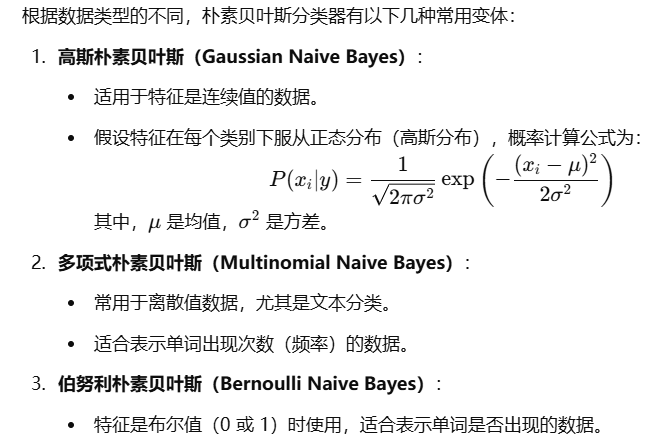
朴素贝叶斯算法 基本思想:
sklearn实现 1 from sklearn.naive_bayes import GaussianNB
GaussianNB()
1 2 clf.fit(iris_x_train,iris_y_train)
GaussianNB()
1 2 3 4 res=clf.predict(iris_x_test) print (res)print (iris_y_test.values)
[0 1 0 0 1 2 1 1 2 1 2 0 2 2 1 0 0 2 0 0 2 2 2 1 1 1 1 2 1 0]
[0 1 0 0 1 2 1 1 2 1 2 0 2 2 1 0 0 2 0 0 2 2 2 1 1 1 1 2 1 0]
1 2 3 accuracy = clf.score(iris_x_test,iris_y_test) print ("预测正确率:{:.0%}" .format (accuracy))
预测正确率:100%
<ipython-input-29-b1c5d7cc9ad0>:25: MatplotlibDeprecationWarning: shading='flat' when X and Y have the same dimensions as C is deprecated since 3.3. Either specify the corners of the quadrilaterals with X and Y, or pass shading='auto', 'nearest' or 'gouraud', or set rcParams['pcolor.shading']. This will become an error two minor releases later.
plt.pcolormesh(t1,t2,y_predict.reshape(x1.shape),cmap=cm_light)
决策树算法 基本思想
1 from sklearn.tree import DecisionTreeClassifier
1 2 3 4 5 6 7 8 9 10 11 12 13 14 clf=AdaBoostClassifier() clf.fit(iris_x_train,iris_y_train) res=clf.predict(iris_x_test) print (res)print (iris_y_test.values)accuracy = clf.score(iris_x_test,iris_y_test) print ("预测正确率:{:.0%}" .format (accuracy))
---------------------------------------------------------------------------
NameError Traceback (most recent call last)
<ipython-input-38-17c5ee30a199> in <module>
1 # 构建分类器对象
----> 2 clf=AdaBoostClassifier()
3
4 #训练
5 clf.fit(iris_x_train,iris_y_train)
NameError: name 'AdaBoostClassifier' is not defined
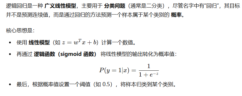
逻辑回归算法
1 2 3 4 5 6 7 8 9 10 11 12 13 14 15 16 17 18 19 from sklearn.linear_model import LogisticRegressionclf=LogisticRegression(solver="saga" ,max_iter=1000 ) clf.fit(iris_x_train,iris_y_train) res=clf.predict(iris_x_test) print (res)print (iris_y_test.values)accuracy = clf.score(iris_x_test,iris_y_test) print ("预测正确率:{:.0%}" .format (accuracy))
支持向量机算法 基本思想
1 from sklearn.svm import SVC
1 2 3 4 5 6 7 8 9 10 11 12 13 14 15 clf=SVC() clf.fit(iris_x_train,iris_y_train) res=clf.predict(iris_x_test) print (res)print (iris_y_test.values)accuracy = clf.score(iris_x_test,iris_y_test) print ("预测正确率:{:.0%}" .format (accuracy))
集成方法——随机森林 基本思想
1 from sklearn.ensemble import RandomForestClassifier
1 2 3 4 5 6 7 8 9 10 11 12 13 14 clf=RandomForestClassifier() clf.fit(iris_x_train,iris_y_train) res=clf.predict(iris_x_test) print (res)print (iris_y_test.values)accuracy = clf.score(iris_x_test,iris_y_test) print ("预测正确率:{:.0%}" .format (accuracy))
集成方法——Adaboost(自适应增强算法)
1 2 3 4 5 6 7 8 9 10 11 12 13 14 15 16 17 18 from sklearn.ensemble import AdaBoostClassifierfrom sklearn.naive_bayes import GaussianNBclf=AdaBoostClassifier() clf.fit(iris_x_train,iris_y_train) res=clf.predict(iris_x_test) print (res)print (iris_y_test.values)accuracy = clf.score(iris_x_test,iris_y_test) print ("预测正确率:{:.0%}" .format (accuracy))
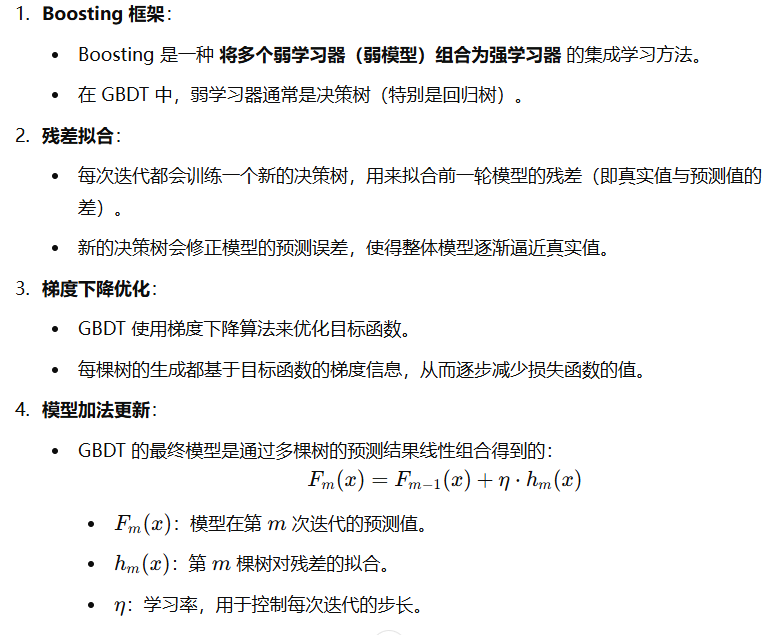
集成方法——梯度提升树GBDT
1 2 3 4 5 6 7 8 9 10 11 12 13 14 15 16 17 18 from sklearn.ensemble import GradientBoostingClassifierclf=GradientBoostingClassifier() clf.fit(iris_x_train,iris_y_train) res=clf.predict(iris_x_test) print (res)print (iris_y_test.values)accuracy = clf.score(iris_x_test,iris_y_test) print ("预测正确率:{:.0%}" .format (accuracy))
大杀器
xgboost
lightgbm
stacking